Abaqus A Deep Dive into FEA

Abaqus, the industry-standard finite element analysis (FEA) software, is way more than just a program; it’s a powerful tool used by engineers across various disciplines to simulate real-world scenarios. From designing skyscrapers that can withstand earthquakes to crafting lightweight yet incredibly strong aerospace components, Abaqus allows engineers to push the boundaries of innovation. This deep dive will explore its core functionalities, applications, and advanced techniques, making you a bona fide Abaqus pro.

We’ll cover everything from the basics of creating finite element models and selecting appropriate material properties to mastering advanced techniques like submodeling and nonlinear analysis. We’ll also compare Abaqus to other popular FEA software and tackle common troubleshooting issues. Get ready to level up your engineering game!

Table of Contents

Abaqus Introduction

Abaqus is a powerful and widely used finite element analysis (FEA) software package employed by engineers and researchers across various industries to simulate the behavior of materials and structures under diverse loading conditions. It’s known for its comprehensive capabilities, robust solver, and extensive material library, making it a go-to tool for complex simulations.Abaqus’s core functionality centers around solving complex engineering problems through FEA.

This involves discretizing a physical system into smaller elements, applying boundary conditions and loads, and then using numerical methods to predict the system’s response. This response can include stress, strain, displacement, temperature, and other relevant physical quantities, providing valuable insights for design optimization and failure prediction. The software excels in handling both linear and nonlinear problems, encompassing various material behaviors and geometric complexities.

Abaqus Modules

Abaqus is structured around several distinct modules, each designed for specific analysis types. These modules allow users to tailor their simulations to their precise needs, avoiding unnecessary computational overhead. The availability and usage of these modules often depend on the specific license purchased.

Standard: This module forms the core of Abaqus, providing capabilities for static, dynamic, and coupled analyses. It’s the foundation upon which many other modules build.
Explicit: This module is specialized for high-speed dynamic events, such as impact, crash, and explosion simulations. It uses an explicit time integration scheme, making it ideal for problems involving large deformations and complex contact interactions.
CFD: The Computational Fluid Dynamics module enables the simulation of fluid flow and heat transfer. This allows for coupled fluid-structure interaction (FSI) analyses, crucial in many engineering applications.
Electromagnetics: This module allows for the simulation of electromagnetic fields and their interaction with structures. This is particularly important in applications involving electrical machines, antennas, and other electromagnetic devices.
Others: Additional modules cater to specific needs like acoustics, fatigue analysis, and optimization studies.

Abaqus Development History

Abaqus’s development began in the 1970s at Hibbitt, Karlsson & Sorensen, Inc. (HKS). Initially focused on providing robust and accurate solutions for linear and nonlinear finite element analysis, Abaqus gradually expanded its capabilities over the decades. Key milestones include the introduction of explicit dynamics, coupled physics simulations, and an increasingly comprehensive material library. The software’s evolution has been driven by advancements in computational power and the ever-growing demands of engineering simulations across various industries.

Simulia, a Dassault Systèmes brand, acquired HKS and continues to develop and maintain Abaqus, ensuring its continued relevance and competitiveness in the FEA market. The software has seen numerous releases over the years, each incorporating new features, improved algorithms, and enhanced user interface elements. This continuous development ensures Abaqus remains a leading FEA tool.

Abaqus Applications in Engineering

Abaqus, a powerful finite element analysis (FEA) software package, finds widespread use across various engineering disciplines. Its ability to simulate complex physical phenomena makes it an invaluable tool for design optimization, problem-solving, and predictive analysis. This section explores some key applications of Abaqus in civil, mechanical, and aerospace engineering.

Abaqus Applications in Civil Engineering

Abaqus is extensively used in civil engineering for analyzing the structural integrity and performance of buildings, bridges, dams, and other infrastructure. Engineers leverage Abaqus to model complex geometries, material properties, and loading conditions to predict structural behavior under various scenarios. For instance, Abaqus can be used to simulate the seismic response of a high-rise building, predict the stress distribution in a bridge under heavy traffic loads, or assess the stability of a dam under extreme hydrological conditions.

This allows engineers to identify potential weaknesses and optimize designs for improved safety and durability. Specific examples include analyzing the impact of ground vibrations on building foundations or simulating the long-term creep and shrinkage of concrete structures.

Abaqus in Mechanical Engineering Design

In mechanical engineering, Abaqus plays a crucial role in designing and optimizing various components and systems. Engineers use it to simulate the mechanical behavior of parts under different loads, temperatures, and environmental conditions. This includes analyzing stress, strain, deformation, and fatigue life. Abaqus enables engineers to assess the performance of components such as gears, bearings, engine parts, and chassis under various operating conditions.

This predictive capability allows for early detection of potential failures, leading to improved designs and reduced prototyping costs. For example, Abaqus could be used to optimize the design of a connecting rod in an engine to minimize weight while ensuring sufficient strength and durability.

Abaqus in Aerospace Engineering Simulations

The aerospace industry relies heavily on Abaqus for simulating the complex loading and environmental conditions experienced by aircraft and spacecraft. Abaqus can be used to model the aerodynamic loads on aircraft wings, the structural response of aircraft fuselages to extreme pressures, and the thermal stresses on spacecraft components during re-entry. It is also used to analyze the impact of fatigue and corrosion on aerospace structures.

The software’s ability to handle nonlinear material behavior and complex boundary conditions makes it particularly well-suited for simulating the demanding environments encountered in aerospace applications. A specific example would be simulating the stress on a turbine blade under high-temperature and high-speed conditions.

Abaqus Applications Across Industries

Industry	Application	Example	Benefits
Civil Engineering	Structural Analysis	Seismic analysis of a high-rise building	Improved design safety and durability; reduced construction costs
Mechanical Engineering	Component Design	Stress analysis of a connecting rod	Optimized design; reduced weight and material usage; improved performance
Aerospace Engineering	Structural Integrity	Analysis of aerodynamic loads on aircraft wings	Enhanced safety; improved design efficiency; reduced risk of failure
Automotive Engineering	Crash Simulation	Impact analysis of a vehicle collision	Improved vehicle safety; optimized crashworthiness design

Abaqus Modeling Techniques

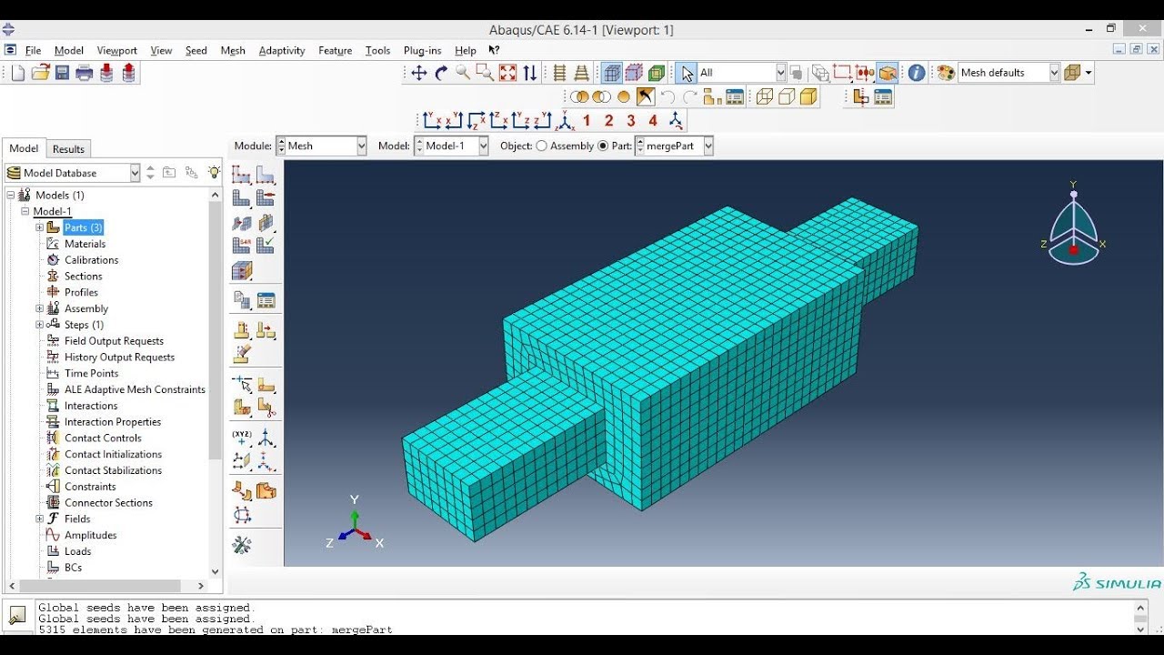
Building a finite element model (FEM) in Abaqus involves a systematic process of translating a real-world engineering problem into a numerical representation that the software can solve. This process allows engineers to simulate the behavior of structures and components under various loading conditions, providing valuable insights into their performance and potential failure modes. Accuracy and efficiency in this process are paramount for reliable simulation results.

The creation of a finite element model in Abaqus typically begins with defining the geometry of the part or assembly. This can be done by importing CAD models or by creating geometry directly within Abaqus/CAE. Next, the model is divided into smaller elements, a process called meshing. Material properties are then assigned to each element, followed by the definition of boundary conditions (constraints) and loads.

Finally, the model is solved using Abaqus/Standard or Abaqus/Explicit, depending on the nature of the analysis. Post-processing then allows for visualization and interpretation of the results.

Meshing Techniques in Abaqus

Meshing is crucial for the accuracy and efficiency of a finite element analysis. The choice of meshing technique significantly impacts the computational cost and the accuracy of the results. A finer mesh generally leads to higher accuracy but increases computational time. A coarser mesh can be computationally efficient but may not capture fine details of the geometry or stress concentrations.

Abaqus offers several meshing techniques, each with its own strengths and weaknesses.

Common techniques include structured meshing, where elements are arranged in a regular pattern, and unstructured meshing, which allows for greater flexibility in adapting to complex geometries. Adaptive meshing automatically refines the mesh in areas of high stress gradients, improving accuracy where it’s needed most. Sweep meshing is particularly useful for creating meshes in complex geometries with rotational symmetry.

The selection of the optimal meshing technique depends on the complexity of the geometry, the desired accuracy, and the available computational resources.

Element Types in Abaqus

Abaqus provides a wide range of element types, each suited to different analysis types and material behaviors. Selecting the appropriate element type is crucial for obtaining accurate and reliable results. Incorrect element selection can lead to inaccurate predictions or even convergence issues.

For example, linear elements are simpler and computationally less expensive but may not accurately capture non-linear behavior. Higher-order elements, such as quadratic elements, offer improved accuracy but increase computational cost. Solid elements are used for three-dimensional analyses, while shell and beam elements are suitable for thin-walled structures and slender members, respectively. The choice of element type also depends on the material model used.

For instance, a hyperelastic material model might require specific element types capable of handling large deformations. For problems involving contact, specialized contact elements are needed to accurately model the interaction between surfaces.

Material Modeling in Abaqus

Choosing the right material model is crucial for accurate and reliable simulation results in Abaqus. The accuracy of your finite element analysis (FEA) hinges on how well the model represents the real-world behavior of the materials involved. This section delves into the various material models available and how to properly define their properties within the Abaqus environment.Material models in Abaqus range from simple linear elastic models to highly complex nonlinear models capable of capturing intricate material behavior.

The selection depends heavily on the specific application and the level of detail required.

Available Material Models

Abaqus offers a vast library of material models categorized by their constitutive behavior. These models account for various physical phenomena like elasticity, plasticity, viscoelasticity, hyperelasticity, creep, and damage. Linear elastic models, for example, are suitable for materials that deform elastically under load and return to their original shape upon unloading. However, many engineering materials exhibit nonlinear behavior, requiring more sophisticated models.

Plasticity models account for permanent deformation, while viscoelastic models incorporate time-dependent effects. Hyperelastic models are used for materials like rubber that undergo large deformations. Creep models capture the time-dependent deformation under constant stress, and damage models simulate material degradation under loading. The choice of model should always be justified based on the material’s known response and the simulation’s objectives.

Defining Material Properties in Abaqus

Defining material properties correctly is just as critical as choosing the appropriate model. This involves inputting parameters that govern the material’s response to loading. For a linear elastic material, this would typically involve specifying Young’s modulus (E) and Poisson’s ratio (ν). More complex models require additional parameters. For example, a plasticity model might need yield strength, hardening parameters, and possibly parameters describing the material’s behavior under different loading conditions (e.g., tension versus compression).

Abaqus provides various ways to define these properties, including directly inputting values, using experimental data to fit the model, or employing built-in material libraries. Accurate property determination often involves experimental testing, and it is important to use appropriate units and ensure consistency throughout the model. For example, if you use MPa for stress, you must also use MPa for Young’s Modulus.

Importance of Material Model Selection

The selection of an appropriate material model significantly impacts the accuracy and reliability of the simulation results. Using an overly simplified model for a complex material can lead to inaccurate predictions, potentially resulting in design flaws or unsafe structures. Conversely, using an overly complex model when a simpler one would suffice can increase computational cost and complexity without necessarily improving the accuracy.

Consider a bridge design: using a simple linear elastic model for the concrete might be sufficient for preliminary stress analysis, but if fatigue and creep effects are important, a more sophisticated viscoelastic or damage model would be necessary. For a crash simulation of a car, hyperelastic models would be needed to capture the large deformations of the rubber components, while plasticity models would be needed for the metallic parts.

The appropriate selection is a balance between accuracy and computational efficiency, driven by a clear understanding of the material behavior and the simulation objectives.

Abaqus Solver and Solution Procedures

Okay, so we’ve covered the basics of Abaqus – modeling, materials, the whole shebang. Now let’s dive into the engine room: the solver and solution procedures. This is where Abaqus crunches the numbers and gives you those sweet, sweet results. Getting this right is crucial for accurate and efficient simulations.The Abaqus solver is the heart of the simulation process, responsible for solving the complex equations that govern the behavior of your model.

Understanding how it works and how to configure it properly is key to getting reliable results. Think of it like the chef in a restaurant; you can have the best ingredients (your model and material properties), but without a skilled chef (the solver), you won’t get a delicious meal (accurate simulation results).

Abaqus Solvers

Abaqus offers a variety of solvers, each designed for different types of analysis. The choice of solver depends heavily on the type of problem you’re solving – linear, nonlinear, static, dynamic, etc. Selecting the wrong solver can lead to inaccurate results or even simulation failure. For example, using a linear solver for a highly nonlinear problem is a recipe for disaster.

Abaqus/Standard uses an implicit solver, known for its stability and accuracy in solving complex nonlinear problems. It’s great for problems involving large deformations or material nonlinearities. Abaqus/Explicit, on the other hand, is an explicit solver, perfect for highly dynamic events like impact or explosions, where speed is paramount. It handles these situations incredibly well, but might not be the best choice for static problems.

Choosing the right solver is like picking the right tool for the job – a hammer isn’t ideal for screwing in a screw.

Setting Up a Solution Procedure

Setting up a solution procedure involves defining the analysis type, specifying the solver, defining the steps in your analysis, and setting the appropriate controls. This process is typically done through the “Step” module in Abaqus/CAE. You’ll define things like the time period for the analysis, the load increments, and the convergence criteria. Imagine building a house; you wouldn’t just throw all the materials together at once.

You’d follow a plan, step by step. Similarly, in Abaqus, you define the steps – each representing a phase in your simulation. For instance, you might have a step for applying a load, followed by a step to analyze the response. These steps are crucial for managing the simulation’s progression and ensuring accurate results. Failure to properly define these steps can result in incomplete or erroneous solutions.

Convergence Criteria

Convergence criteria are essential for ensuring the accuracy and reliability of your simulation. They define the acceptable level of error in the solution. Abaqus iteratively solves the equations governing your model, and these criteria determine when the solution is considered “good enough” to stop iterating. Common convergence criteria include energy convergence, force convergence, and displacement convergence. Think of it like baking a cake; you wouldn’t stop baking just because itlooks* done; you’d check the internal temperature (convergence criteria) to ensure it’s cooked through.

If the solver doesn’t meet the specified criteria, it indicates potential problems, such as an inadequate mesh, incorrect boundary conditions, or an inappropriate material model. Ignoring convergence warnings can lead to inaccurate or completely unreliable results. A common issue is that the solver might fail to converge if the load is applied too quickly or the mesh is too coarse.

Adjusting the load application or refining the mesh can often resolve these issues.

Post-Processing and Results Interpretation in Abaqus

Okay, so you’ve run your Abaqus simulation – congrats! Now comes the fun part: figuring out what all those numbers and graphs actuallymean*. Post-processing in Abaqus is all about visualizing and analyzing the results of your finite element analysis (FEA) to understand how your model behaved under the applied loads and conditions. It’s like being a digital detective, piecing together the story of your simulation.Post-processing in Abaqus involves a variety of tools to extract meaningful insights from your simulation data.

This allows engineers to validate their designs, optimize performance, and troubleshoot potential problems before they occur in the real world. Effective post-processing is crucial for translating raw simulation data into actionable engineering knowledge.

Available Post-Processing Tools in Abaqus

Abaqus offers a powerful suite of visualization and data extraction tools. These tools allow for detailed examination of results, ranging from simple plots to complex contour plots and animations. Key tools include the Visualization module, which provides interactive graphical representations of results; the XY Data module, useful for generating plots of specific data points; and the Report module, which allows the creation of customized reports summarizing key simulation results.

Beyond these core tools, Abaqus also integrates with scripting languages like Python, providing further customization and automation capabilities for advanced post-processing tasks.

Interpreting Results from Abaqus Simulations

Interpreting Abaqus results requires a solid understanding of both the simulation setup and the fundamental principles of FEA. It’s not just about looking at pretty pictures; it’s about understanding what those pictures represent in the context of your engineering problem. For example, high stress concentrations might indicate potential failure points in a design, while large displacements could suggest a need for structural reinforcement.

Always compare your results against expected behavior, considering factors like material properties, boundary conditions, and loading scenarios. Discrepancies might point to errors in the model or the need for further refinement.

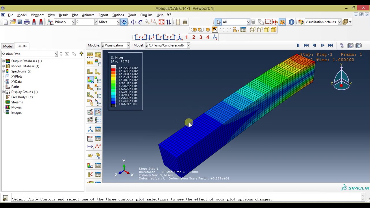
Visualizing Stress, Strain, and Displacement Results

Let’s look at how to visualize some common results. Imagine a simple cantilever beam subjected to a point load at its free end.

Stress Visualization

A contour plot of von Mises stress would show the highest stress concentrations at the fixed end of the beam and potentially near the point load application. The color scale would indicate the magnitude of stress, with red typically representing the highest stress levels and blue representing the lowest. This visualization helps identify potential failure locations based on the material’s yield strength.

You might see a smooth gradient of stress distribution, or potentially sharp peaks indicating stress concentrations, which could warrant design modifications.

Strain Visualization

Similarly, a contour plot of strain would show the regions experiencing the most deformation. Again, a color scale would illustrate the magnitude of strain, with high strain areas indicating significant deformation. This is particularly useful for identifying areas prone to yielding or fracture. Comparing stress and strain visualizations can help pinpoint locations where material failure is most likely.

Displacement Visualization

Displacement results can be visualized using deformed shape plots. The deformed shape shows the actual displacement of the nodes in the model. This allows you to see the overall deflection of the beam under load. You could exaggerate the displacement for better visualization. By comparing the deformed shape to the undeformed geometry, you can easily assess the magnitude and direction of the displacement at various points along the beam.

This is critical for assessing structural integrity and functionality.

Abaqus Scripting and Customization

Abaqus’s power extends far beyond its graphical user interface (GUI). By leveraging Python scripting, users can dramatically increase efficiency, automate repetitive tasks, and customize workflows to fit their specific needs. This opens up a world of possibilities for advanced users and engineers seeking to streamline their analysis processes. This section will explore the capabilities of Abaqus scripting and provide examples of its practical applications.Python’s integration with Abaqus provides a robust and flexible framework for automating various aspects of the finite element analysis (FEA) process.

From model creation and meshing to running analyses and post-processing results, Python scripts can handle many steps, significantly reducing manual effort and potential for human error. This allows for greater control over the analysis and enables the creation of custom tools tailored to specific engineering problems.

Abaqus simulations generate tons of data – input files, results, and those pesky journal files. Keeping everything organized can be a nightmare, which is why a solid document management system is key. Properly managing your Abaqus projects ensures you can easily find what you need, especially when revisiting older analyses or collaborating with others on a project.

Efficient file management ultimately saves you time and frustration with Abaqus.

Python Scripting in Abaqus

Abaqus’s Python scripting environment allows users to interact directly with the software’s internal objects and functions. This means you can programmatically create models, define materials, apply loads and boundary conditions, run simulations, and extract results—all without touching the mouse. The Abaqus Scripting Interface (ASI) provides access to a comprehensive library of functions and classes, enabling complex automation and customization.

For instance, you can write scripts to generate models based on parameters read from external files, or create custom post-processing tools to visualize and analyze results in a specific manner. The use of loops and conditional statements allows for complex logic within scripts, enabling sophisticated automation and adaptation to varying analysis needs.

Automating Tasks Using Abaqus Scripting

One of the most significant advantages of Abaqus scripting is its ability to automate repetitive tasks. Consider a scenario where you need to run a series of analyses with slightly different parameters. Manually changing these parameters for each analysis is tedious and error-prone. A Python script can easily automate this process. The script can iterate through a range of parameters, create a model for each parameter set, run the analysis, and store the results.

This approach saves significant time and reduces the risk of human error. Another example is batch processing of multiple CAD models. A script can automatically import, mesh, and analyze numerous models, consolidating the results into a single report.

Customizing Abaqus Workflows Through Scripting

Abaqus scripting allows for deep customization of workflows. Imagine you need a specific post-processing routine that’s not available in Abaqus’s built-in tools. A Python script can be written to perform this custom routine, extracting the required data and generating the desired visualizations. For example, a script could be created to automatically generate contour plots of stress and strain for specific regions of interest within a complex model, or it could automatically generate customized reports summarizing key results for various analyses.

Similarly, you could create a script to automate the process of creating and running optimization studies by systematically modifying design parameters and evaluating the resulting performance. This level of customization allows engineers to tailor Abaqus to their specific needs and work styles, ultimately leading to more efficient and effective engineering analysis.

Advanced Abaqus Techniques

Okay, so we’ve covered the basics of Abaqus. Now let’s dive into some seriously powerful stuff – the advanced techniques that let you tackle complex engineering problems. We’ll explore submodeling, co-simulation, nonlinear analysis, and dynamic analysis, showing you how Abaqus can handle the really tough simulations.Submodeling and co-simulation are two crucial techniques for tackling models that are too large or computationally expensive to solve in a single run.

Nonlinear analysis expands Abaqus’ capabilities to handle materials and structures that behave in non-linear ways, which is pretty much everything in the real world. Finally, dynamic analysis allows us to model things that move and change over time, from earthquakes to car crashes.

Submodeling

Submodeling lets you focus on a small, critical region of a larger model. Imagine you’re analyzing a weld in a large structure. Instead of running a massive simulation of the entire structure, you can create a smaller, highly refined submodel around the weld. This submodel uses the results from a coarser simulation of the entire structure as boundary conditions.

This approach significantly reduces computation time while maintaining accuracy in the area of interest. The boundary conditions from the global model are applied to the edges of the submodel, essentially creating a “zoom” effect on the region requiring more detailed analysis. Think of it like using a high-powered microscope to examine a specific detail while still understanding its context within the larger picture.

The accuracy of the submodel depends heavily on the mesh refinement in the submodel region and the accuracy of the global model’s results used as boundary conditions.

Co-simulation

Co-simulation is all about linking different simulation tools together. Maybe you’re analyzing a system with fluid flow and structural deformation, like a bridge pier in a river. You might use a Computational Fluid Dynamics (CFD) software for the fluid and Abaqus for the structure. Co-simulation lets you exchange data between these programs, allowing the fluid forces to influence the structural response and vice-versa.

This integrated approach is much more realistic than analyzing each part in isolation. The key here is careful consideration of data exchange formats and ensuring compatibility between the different software packages. A common approach is to use a coupling algorithm to manage the iterative exchange of data between the simulations, ensuring convergence and stability of the coupled solution.

Nonlinear Analysis

Nonlinear analysis is where things get interesting. Linear analysis assumes a proportional relationship between load and displacement – double the load, double the displacement. But in the real world, materials often exhibit nonlinear behavior. Think about a rubber band – it stretches more easily as it gets longer. Abaqus handles this using sophisticated material models that account for plasticity, creep, hyperelasticity, and more.

Nonlinear analysis requires iterative solution procedures, as the stiffness of the structure changes with deformation. This means more computational time, but it’s essential for accurate results in many engineering applications, such as predicting the failure of a component under extreme loading conditions. For example, a car crash simulation would absolutely require nonlinear analysis to accurately model the plastic deformation of the vehicle’s body.

Dynamic Analysis

Dynamic analysis models systems that change over time. This includes things like vibrations, impacts, and explosions. Abaqus offers various dynamic analysis techniques, including explicit and implicit methods. Explicit dynamics is best for short-duration, high-velocity events like impacts, because it uses a small time step and directly integrates the equations of motion. Implicit dynamics, on the other hand, is better suited for longer-duration events, as it uses a larger time step and solves a system of equations at each time step.

The choice between explicit and implicit methods depends on the specific problem being analyzed. For instance, a simulation of a bird strike on an aircraft would likely use explicit dynamics due to the short duration and high impact forces, while the analysis of a building’s response to an earthquake might utilize implicit dynamics due to the longer duration of the event.

Abaqus vs. Other FEA Software

Choosing the right FEA software depends heavily on your specific needs and project requirements. While Abaqus is a powerful and versatile tool, it’s not necessarily the best choice for every application. This section compares Abaqus to other popular FEA packages, highlighting its strengths and weaknesses in relation to its competitors. We’ll focus on key features to help you understand the nuances of each software and make an informed decision.

Direct comparison between FEA software packages can be tricky, as the “best” software is highly context-dependent. Factors like project size, material complexity, desired level of accuracy, budget, and available expertise all play a crucial role. However, we can identify general trends and common strengths and weaknesses to aid in the selection process.

Abaqus Feature Comparison

The following table compares Abaqus with two other commonly used FEA packages: ANSYS and COMSOL. Note that this is not an exhaustive comparison, and the specific features and capabilities of each software can vary depending on the modules and licenses acquired.

Feature	Abaqus	ANSYS	COMSOL
Nonlinear Analysis Capabilities	Excellent; robust handling of large deformations, contact, and material nonlinearities. Widely used for complex material models.	Strong capabilities; offers a broad range of nonlinear solvers and material models.	Very strong; excels in multiphysics simulations where nonlinear behavior is often present.
Explicit Dynamics	Powerful explicit solver for high-speed impact and crash simulations.	Offers both explicit and implicit dynamic solvers.	Explicit capabilities available but generally not as comprehensive as Abaqus or ANSYS.
Linear Analysis Capabilities	Comprehensive linear analysis capabilities, covering a wide range of applications.	Strong linear analysis capabilities, widely considered industry standard.	Good linear analysis capabilities, particularly strong in coupled physics problems.
Multiphysics Capabilities	Growing capabilities through add-on modules, but not as comprehensive as COMSOL.	Offers multiphysics capabilities through various add-on modules.	Industry-leading multiphysics capabilities, allowing for the simulation of coupled physical phenomena.
Ease of Use	Steeper learning curve than some competitors; requires a strong understanding of FEA principles.	Relatively user-friendly interface, with a large user base and extensive online resources.	User-friendly interface, especially for users familiar with MATLAB-like scripting.
Cost	Generally expensive, especially with add-on modules.	Can be expensive, depending on the modules selected.	Can be expensive, particularly for comprehensive multiphysics simulations.
Customization and Scripting	Powerful scripting capabilities using Python, allowing for extensive customization.	Offers scripting capabilities, but potentially less flexible than Abaqus.	Strong scripting capabilities using its own scripting language.

Troubleshooting Common Abaqus Issues

Let’s face it, Abaqus, despite its power, can throw some curveballs. This section dives into common problems you might encounter and provides practical solutions to get your simulations running smoothly. We’ll cover error messages, convergence issues, and modeling best practices to prevent headaches down the line.

Common Abaqus Error Messages and Their Solutions

Understanding Abaqus error messages is crucial for efficient troubleshooting. These messages often pinpoint the source of the problem, but deciphering them can be tricky. Here are some frequently encountered errors and their potential fixes.

“Too many iterations” error: This usually indicates a convergence problem. Check your model for overly-constrained parts, overly-large load steps, or inappropriate material properties. Try reducing the load step size, refining the mesh, or adjusting the solver parameters.
“Singular matrix” error: This suggests your model is either under-constrained (lacks sufficient boundary conditions) or has elements with zero volume (meshing issues). Review your boundary conditions and check for any distorted or overlapping elements in your mesh.
“Negative Jacobian” error: This indicates that the element is inverted or severely distorted. This is a meshing problem; refine your mesh in the area where the error occurs, and ensure that elements are not excessively distorted.
“Out of memory” error: This means your simulation requires more RAM than available. Try reducing the model size, refining the mesh less aggressively, or using a more efficient solver. You might also need to increase the RAM on your computer.

Convergence Problems in Abaqus Simulations

Convergence problems are a common frustration in FEA. These often manifest as errors like “too many iterations” or unexpected results. Addressing these requires a systematic approach.

Mesh Refinement: A finer mesh generally improves accuracy but increases computational cost. Focus refinement on areas of high stress gradients or geometric complexity.
Load Step Size Reduction: Smaller load steps can help the solver find a solution, especially for nonlinear problems. Start with smaller increments and gradually increase them if convergence is achieved.
Solver Parameter Adjustment: Abaqus offers various solver parameters that can affect convergence. Experimenting with these parameters (e.g., automatic incrementation, solution controls) can significantly improve convergence behavior.
Material Model Selection: Choosing an appropriate material model is critical. An inappropriate model might lead to non-convergence or inaccurate results. Consider the material’s behavior under load and select a model that reflects this accurately.

Best Practices for Avoiding Common Abaqus Modeling Mistakes

Proactive measures can significantly reduce the likelihood of encountering errors. These best practices help create robust and reliable models.

Proper Meshing: Use appropriate element types and mesh densities. Avoid overly distorted or excessively skewed elements. Mesh refinement should be strategic, focusing on areas of high stress concentration.
Accurate Boundary Conditions: Carefully define boundary conditions to realistically represent the physical constraints of the problem. Ensure that the model is adequately constrained to prevent rigid body motion.
Realistic Material Properties: Use accurate material properties obtained from experimental data or reliable sources. Inaccurate material data can lead to significant errors in the results.
Verification and Validation: Always verify your model setup and validate your results against analytical solutions or experimental data whenever possible. This ensures the accuracy and reliability of your simulations.
Incremental Loading: Apply loads incrementally, especially for nonlinear problems. This helps the solver converge more smoothly and avoid unexpected behavior.

Conclusion: Abaqus

So, there you have it – a comprehensive look at the world of Abaqus. Whether you’re a seasoned engineer or just starting your FEA journey, understanding Abaqus’ capabilities is crucial in today’s engineering landscape. From its historical development to its cutting-edge applications, Abaqus continues to be a driving force in innovation, allowing engineers to solve complex problems and design the next generation of structures and machines.

Now go forth and conquer those simulations!

Questions and Answers

What’s the difference between Abaqus/Standard and Abaqus/Explicit?

Abaqus/Standard uses an implicit solver, ideal for static and quasi-static analyses, while Abaqus/Explicit uses an explicit solver, perfect for high-speed impact and dynamic events. Think of it like this: Standard is for slow and steady problems, Explicit for the fast and furious ones.

How steep is the learning curve for Abaqus?

It’s definitely not a walk in the park, but plenty of resources exist, including tutorials, online courses, and excellent documentation. Start with the basics, build a solid foundation, and don’t be afraid to experiment!

Can Abaqus handle large models?

Yes, but efficiently handling large models often requires advanced techniques like submodeling and parallel processing to manage computational resources and time effectively.

Is Abaqus only for experienced engineers?

Nope! While mastering advanced features takes time, the fundamentals are accessible to anyone with a basic understanding of engineering principles and numerical methods. Plenty of introductory resources are available.

Where can I find Abaqus support?

Simulia (the creators of Abaqus) offers various support options, including online documentation, training courses, and direct support channels. The Abaqus user community also provides a wealth of knowledge and assistance.